Vector Functions

>

restart:

Se e: Stewart, chapter 13. We start with loading the package VectorCalculus :

>	with(VectorCalculus):

A vector function   r (t) can be defined as follows:

>	r:= t -> < x(t), y(t), z(t) >;

The output looks a little bit strange, but calling the function generates the expected result:

>

r(t);

Then the velocity  vector v (t) and the acceleration  vector a (t) are given by:

>	v := t -> diff(r(t),t);

>	a := t -> diff(v(t),t);

Again this is what we want, since:

>	v(t); a(t);

Now, for instance, we can compute the arc length  of a curve given by r (t) with  and  :

>	L:=ArcLength(r(t),t=a..b);

Now consider example 4 of § 13.1. That the curve given by the vector function

>	r:=t-><cos(t),sin(t),t>: r(t);

represents a helix  can be seen by using the command SpaceCurve , which is included in the package VectorCalculus  since Maple 11. In Maple 10 this command was only available in the package Student[VectorCalculus] . Explore the numerous options (such as different views) when you select the picture by a mouse click!

>	SpaceCurve(r(t),t=0..6*Pi);

In example 6 of § 13.1 a vector function is obtained that represents the intersection of the cylinder  and the plane  :

>	with(plots): P1:=implicitplot3d({x^2+y^2=1,y+z=2},x=-2..2,y=-2..2,z=-2..4,orientation=[45,60]): display(P1);

The vector function representing the curve of intersection is:

>	r:=t-><cos(t),sin(t),2-sin(t)>: r(t);

>	P2:=SpaceCurve(r(t),t=0..2*Pi,color=red,thickness=5): display(P2);

If we display the cylinder, the plane and the intersecting curve into one figure we see that it seems to be correct (again get different views by clicking the picture!):

>	display(P1,P2);

The toroidal spiral in figure 7 of §  13.1 can be created as follows:

>	SpaceCurve(<(4+sin(20*t))*cos(t),(4+sin(20*t))*sin(t),cos(20*t)>,t=0..2*Pi,numpoints=1000);

and the trefoil knot in figure 8 of § 13.1:

>	SpaceCurve(<(2+cos(1.5*t))*cos(t),(2+cos(1.5*t))*sin(t),sin(1.5*t)>,t=0..6*Pi,numpoints=1000);

In example 1 of § 13.3 the arc length  of the helix given by

>	r:=t-><cos(t),sin(t),t>: r(t);

is derived:

>	L:=ArcLength(r(t),t=0..2*Pi);

We can also compute the curvature  of this curve:

>	Curvature(r(t));

>	simplify(%);

Example 3 of § 13.3, the curvature of a circle with radius  :

>	Curvature(<a*cos(t),a*sin(t)>) assuming a::constant, a::positive;

>	simplify(%);

Therefore  is often called the radius of curvature :

>	RadiusOfCurvature(<a*cos(t),a*sin(t)>) assuming a::constant, a::positive;

Example 4 of § 13.3:

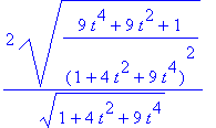
>	simplify(Curvature(<t,t^2,t^3>));

>	subs(t=0,%);

Example 5 of §  13.3:

>	simplify(Curvature(<x,x^2>)) assuming x::real;

Example 6 of §  13.3. We reconsider the circular helix:

>

r(t);

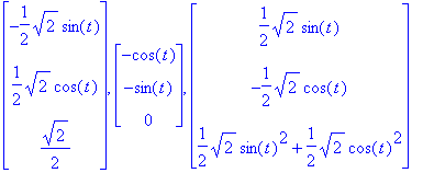
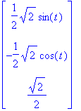
The unit tangent vector   T (t), the principal unit normal vector   N (t) and the binormal vector   B (t) together form the so-called TNB frame (or Frenet frame):

>	TNBFrame(r(t));

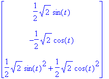
Note that the binormal vector B (t) can be simplified. This can be done by first isolating this vector:

>	TNBFrame(r(t),'output'=['B']);

>	simplify(%);

>